The study of the dynamical properties of time series is key to a variety of research areas, such as ecology and finance, where correctly identifying past or anticipating impending occurrences of temporal abrupt shifts is essential to understanding the temporal stability of a given variable.
This is a tutorial about a simple and straightforward time series classification approach based on their shape and trend. The approach classifies time series into abrupt and non-abrupt (constant, linear, nonlinear) trajectories by combining several existing methods following CITE. It also allows for assessing the classification reliability with three independent metrics. By the end of this tutorial you will hopefully know how to:
- Install the necessary packages and R scripts to perform the classification
- Classify individual time series
- Classify time series libraries
- Quantify the classification’s reliability
- Visualize outputs
Import required libraries
library(dplyr)
library(tidyverse)
library(patchwork)
library(cowplot, warn.conflicts=FALSE)
library(MuMIn) %>% suppressMessages()
library(chngpt) %>% suppressMessages()
library(ggtext)
library(pheatmap)
library(ggstatsplot)
library(asdetect) # devtools::install_github("caboulton/asdetect")
library(ggradar) # devtools::install_github("ricardo-bion/ggradar")
library(pracma)
library(MatrixModels)
setwd("~/Documents/biodicee/fish@risk")
source("code/functions_trajclass.R")
load("sim_data.RData") #dataset with time series examples
Single time series example 1
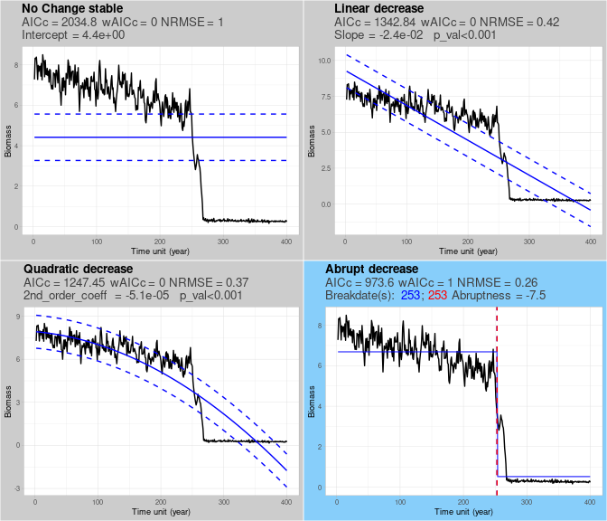
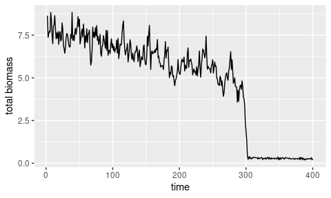
In this example we will use a single time series generated using a modified Ricker’s model following CITE. The time series exhibits an abrupt shift when the system undergoes through a fold bifurcation.
  single.time.series1 <- simu_data %>% filter(sr == noise_df$sr[4],expected_class == "abrupt",iter == 10) %>% select(scen,year,TB) ### extract one time series from database

  p1 <- ggplot()+
  geom_line(data=single.time.series1, aes(x=year, y=TB))+xlab("time")+ylab("total biomass")
  p1
The time series to be classified needs to be a data frame with at least three columns (time series id, time and value). Now let’s apply the classifier to a time series using the following function:
single.classification <- traj_class(prep_data(single.time.series1,type = "data", apriori = FALSE), str = "aic_asd", abr_mtd = c("chg","asd"), asd_chk = TRUE,asd_thr = 0.15, smooth_signif=TRUE, two_bkps=FALSE, run_loo=FALSE, showplots=TRUE, outplot = TRUE)

single.classification$class_plot
The output of this function is the list single.classification, which contains the output plot we see above. In the example we see a time series correctly classified as “abrupt”. Each of the four panels describes the shape and trend of the trajectory: the same timeseries is shown (black line) with a different fit (solid blue line) and standard deviation (dashed lines for all panels except “abrupt” fit). In the “abrupt” panel, the location of breakpoints is indicated by vertical dashed lines. Panel subtitles show AICc score, AICc weight (wAICc), and normalized root mean square error (NRMSE). Trajectory-specific values are also displayed: the intercept of the “no change” model, the slope and associated p-value of the linear model, the second order coefficient and associated p-value of the quadratic model, the location of breakpoints (in blue and red from chngpt and asdetect methods, respectively) and abruptness (the standardized magnitude of the abrupt shift).
Single time series example 2
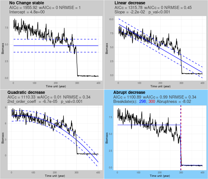
In this second example we will a use a single time series generated using the same model, however in this range of parameters the time series follows a decreasing quadratic trend (for details see CITE).
  single.time.series2 <- simu_data %>% filter(sr == noise_df$sr[3],expected_class == "quadraticA",iter == 18,year<200) %>% select(scen,year,TB) ### extract one time series from database

  p1 <- ggplot()+
  geom_line(data=single.time.series2, aes(x=year, y=TB))+xlab("time")+ylab("total biomass")
  p1

In this case we will use a further metric to measure the quality of the fit using a losing one out method (LOO). For this we set the parameter run_loo = TRUE in the traj_class function. The output of the classifier will be slightly different to the one from the previous example:
single.classification <- traj_class(prep_data(single.time.series2,type = "data", apriori = FALSE), str = "aic_asd", abr_mtd = c("chg","asd"), asd_chk = TRUE,asd_thr = 0.15, smooth_signif=TRUE, two_bkps=FALSE, run_loo=TRUE, showplots=TRUE, outplot = TRUE)

single.classification$class_plot
In this case the time series is correctly classified as quadratic. When applying the LOO method, timepoints that if removed in the LOO process result in a specific shape are highlighted by orange dots in the corresponding panel. In this example, all orange timepoints are displayed on the quadratic panel because when any of them is removed the quadratic shape remains the best fitting one.
Classifying a set of time series
This classification approach can easily be applied to large data sets. In this tutorial we will classify a set of 54 time series with different shapes (9 abrupt, 18 quadratic, 9 linear and 18 no change). For this we can use the function
set.time.series <- simu_data %>% filter(sr == noise_df$sr[4],iter < 10) %>% select(id,year,TB) ### extract one time series from database

set.time.series.list <- split(set.time.series,set.time.series$id)

set.classification <- run_classif_data(set.time.series.list,str = "aic_asd",asd_thr = 0.15,run_loo = FALSE,two_bkps = FALSE,smooth_signif = TRUE,group = "id",time = "year",variable = "TB",outplot = TRUE,save_plot = FALSE)
## [1] "10/54"
## [1] "20/54"
## [1] "30/54"
## [1] "40/54"
## [1] "50/54"
table(set.classification$traj_ts_full$class)
##
## no_change    linear quadratic    abrupt
##        12         5        31         6
set.classification$outlist$`l400_lin_pos_F2-4_r1.0_H0.75_iter08_se0_sr0.05_su0_jfr0_jsz0`$class_plot